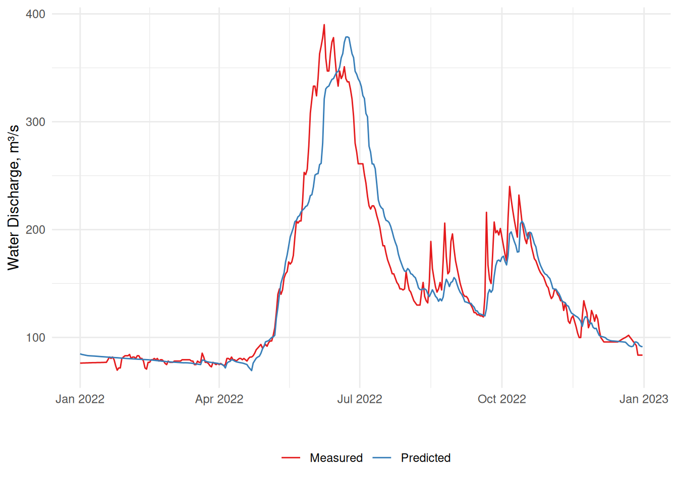
The package includes the mean daily water discharge values (obs in m³/s) measured at the state gauging station Avacha River — Elizovo City (site No. 2090). Alongside the measured water discharge, the mean water discharge in the last 24 hours derived from the GloFAS-ERA5 v4.0 reanalysis is provided (sim).
Example usage
One can estimate the desired metrics using the tidyverse syntax. For example, to get the Nash-Sutcliffe Efficiency (\(NSE\)) or Modified Kling-Gupta Efficiency (\(KGE'\)) for the avacha dataset, one can run:
nse(avacha, obs, sim)
#> # A tibble: 1 × 3
#>   .metric .estimator .estimate
#>   <chr>   <chr>          <dbl>
#> 1 nse     standard       0.895
kge2012(avacha, obs, sim)
#> # A tibble: 1 × 3
#>   .metric .estimator .estimate
#>   <chr>   <chr>          <dbl>
#> 1 kge2012 standard       0.947
Or using the yardstick helper functions, one can create a metric set, combining it with other yardstick metrics, such as \(R^2\):
library(yardstick)
hydro_metrics <- metric_set(kge, pbias, rsq)
hydro_metrics(avacha, obs, sim)
#> # A tibble: 3 × 3
#>   .metric .estimator .estimate
#>   <chr>   <chr>          <dbl>
#> 1 kge     standard      0.947
#> 2 pbias   standard      0.0540
#> 3 rsq     standard      0.898
Such syntax is particularly useful when running a group analysis, for example, estimating model performance for different months:
library(lubridate)
library(dplyr)

avacha |>
  mutate(month = month(date)) |>
  group_by(month) |>
  nse(obs, sim)
#> # A tibble: 12 × 4
#>    month .metric .estimator .estimate
#>    <dbl> <chr>   <chr>          <dbl>
#>  1     1 nse     standard    -2.78
#>  2     2 nse     standard     0.180
#>  3     3 nse     standard     0.0335
#>  4     4 nse     standard    -0.00438
#>  5     5 nse     standard     0.815
#>  6     6 nse     standard    -2.78
#>  7     7 nse     standard    -0.244
#>  8     8 nse     standard    -0.228
#>  9     9 nse     standard     0.359
#> 10    10 nse     standard     0.466
#> 11    11 nse     standard     0.439
#> 12    12 nse     standard     0.455
Alternatively, one can still use the vectorised versions of the metrics, ending with the *_vec suffix:
nse_vec(truth = avacha$obs, estimate = avacha$sim)
#> [1] 0.895008