1) Disclaimer & Preprocessing logic
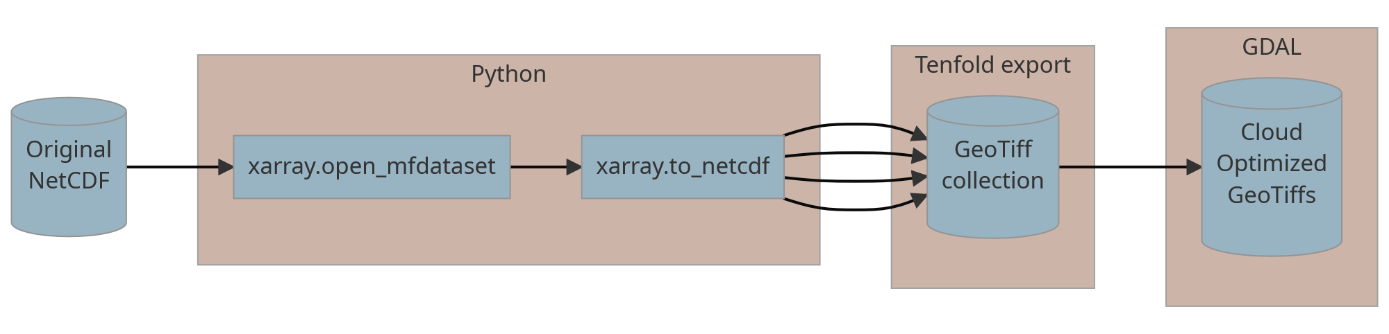
Beneath is the example how can one download and preprocess HBV parameter maps created by Beck et al. (2020). The initial dataset was distributed as NetCDF file. The package provides an opportunity to retreive original (v0.8) and revised (v0.9) versions of the datasets. The v0.8 version contains ten cross-validation folds of 12 parameters:
- BETA – Shape coefficient of recharge function
- FC – Maximum soil moisture storage (mm)
- K0 – Recession coefficient of upper zone (day−1)
- K1 – Recession coefficient of upper zone (day−1)
- K2 – Recession coefficient of lower zone (day−1)
- LP – Soil moisture value above which actual evaporation reaches potential evaporation
- PERC – Maximum percolation to lower zone (mm day−1)
- UZL – Threshold parameter for extra outflow from upper zone (mm)
- TT – Threshold temperature (°C)
- CFMAX – Degree‐day factor (mm °−11 day−1)
- CFR – Refreezing coefficient
- CWH – Water holding capacity
In the v0.9 version authors added four more parameters:
- MAXBAS – base of the triangular routing function (days)
- SFCF – Snowfall correction factor (-)
- PCORR – general precipitation correction factor (-)
- CET – potential evaporation correction factor (-)
We converted every fold to the Cloud-Optimized GeoTiff (COG) using
the following GDAL command:
gdal_translate ordinary.tif COG.tiff -co COPY_SRC_OVERVIEWS=YES -co COMPRESS=LZW -co TILED=YES.
The final COG was validated using the python script.
Thus we ended up with 10 COGs with 12 bands each.
2) Example workflow
The essential aim of the hbv_get_parameters function is
to ease the accessibility of HBV parameter maps created by Beck et
al. (2020). Therefore this
function allows to download any of the cross-validation folds for your
particular area of interest (AOI).
Let’s imagine, you need to download first, second and fifth folds for the Luxembourg.
library(HBVr)
#> Loading required package: terra
#> terra 1.7.3
# library(tmap) # for vizualisztion purposes
# library(sf) # for vizualisztion purposes

# Locate the shapefile
f <- system.file("ex/lux.shp", package="terra")
# Read it as SpatVector
v <- vect(f)

# Plot it!
# tmap_mode("view")
#
# tm_basemap("Stamen.Terrain") +
#   tm_shape(st_as_sf(v)) +
#   tm_polygons()
Initially, the hbv_get_parameters function has two types
of output. First is the mean zonal statistics which is computed with
terra::global in the background. Second one is the simple
SpatRaster output.
To download 1, 2 and 5 folds we need to specify it in the function. Here is the example how can we retrieve mean values for the entire Luxembourg.
zonal_stat <-
  hbv_get_parameters(
    AOI = v,
    folds = c(1, 2, 5),
    mean = TRUE
  )
#> Downloading rasters...
#> Cropping rasters...
The output of zonal_stat is hidden below ↓
zonal_stat
#> $fold_0
#>                mean
#> BETA     3.59133975
#> CET      0.00000000
#> CFMAX    4.76274042
#> CFR      0.02329523
#> CWH      0.03688424
#> FC     557.79513737
#> K0       0.11312447
#> K1       0.22010622
#> K2       0.14379373
#> LP       0.78630368
#> MAXBAS   1.80986611
#> PCORR    1.00000000
#> PERC     3.55778855
#> SFCF     1.00000000
#> TT      -0.06733536
#> UZL     56.14696222
#>
#> $fold_1
#>                 mean
#> BETA    5.235857e+00
#> CET     0.000000e+00
#> CFMAX   2.665556e+00
#> CFR     2.929959e-04
#> CWH     6.203691e-04
#> FC      6.595314e+02
#> K0      9.967822e-02
#> K1      2.003403e-01
#> K2      1.708671e-01
#> LP      9.336371e-01
#> MAXBAS  2.038171e+00
#> PCORR   1.000000e+00
#> PERC    3.316196e-01
#> SFCF    1.000000e+00
#> TT     -2.557204e-01
#> UZL     5.925521e+01
#>
#> $fold_4
#>                mean
#> BETA   4.567642e+00
#> CET    0.000000e+00
#> CFMAX  3.155823e+00
#> CFR    3.054426e-02
#> CWH    3.499128e-05
#> FC     5.611259e+02
#> K0     5.050571e-02
#> K1     2.136054e-01
#> K2     1.490991e-01
#> LP     8.979798e-01
#> MAXBAS 1.969578e+00
#> PCORR  1.000000e+00
#> PERC   2.001591e+00
#> SFCF   1.000000e+00
#> TT     1.804570e-01
#> UZL    9.997002e+01
To download SpatRaster objects we need to run the
following code chunk:
rasters <-
  hbv_get_parameters(
    AOI = v,
    folds = c(1, 2, 5),
    mean = FALSE
  )
#> Downloading rasters...
#> Cropping rasters...
#> Projecting rasters...
The output of rasters is hidden below ↓
rasters
#> $fold_0
#> class : SpatRaster
#> dimensions : 8, 8, 16 (nrow, ncol, nlyr)
#> resolution : 0.1, 0.1 (x, y)
#> extent : 5.7, 6.5, 49.4, 50.2 (xmin, xmax, ymin, ymax)
#> coord. ref. : +proj=longlat +datum=WGS84 +no_defs
#> source(s) : memory
#> names : BETA, CET, CFMAX, CFR, CWH, FC, ...
#> min values : 2.750727, 0, 4.120560, 0.02307616, 0.03650405, 526.2200, ...
#> max values : 4.076468, 0, 5.260039, 0.02346940, 0.03710934, 596.8556, ...
#>
#> $fold_1
#> class : SpatRaster
#> dimensions : 8, 8, 16 (nrow, ncol, nlyr)
#> resolution : 0.1, 0.1 (x, y)
#> extent : 5.7, 6.5, 49.4, 50.2 (xmin, xmax, ymin, ymax)
#> coord. ref. : +proj=longlat +datum=WGS84 +no_defs
#> source(s) : memory
#> names : BETA, CET, CFMAX, CFR, CWH, FC, ...
#> min values : 3.752313, 0, 2.646058, 0.000000000, 0.0005433661, 595.1489, ...
#> max values : 6.000000, 0, 2.686393, 0.001583559, 0.0007155714, 726.9780, ...
#>
#> $fold_4
#> class : SpatRaster
#> dimensions : 8, 8, 16 (nrow, ncol, nlyr)
#> resolution : 0.1, 0.1 (x, y)
#> extent : 5.7, 6.5, 49.4, 50.2 (xmin, xmax, ymin, ymax)
#> coord. ref. : +proj=longlat +datum=WGS84 +no_defs
#> source(s) : memory
#> names : BETA, CET, CFMAX, CFR, CWH, FC, ...
#> min values : 3.373822, 0, 3.016764, 0.03044694, 2.118881e-05, 501.1906, ...
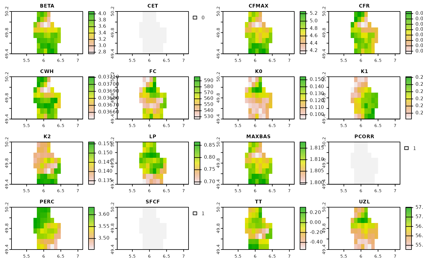
#> max values : 5.262473, 0, 3.247912, 0.03059574, 5.475432e-05, 623.8236, ...The function returns a list of SpatRaster objects. The
first one, i.e. Fold 1, can be plotted like this:
plot(rasters[[1]])